# A tibble: 6 × 5
  Slide_Label case_difficulty Pathologist AI_status  diagnosis_time
  <chr>       <chr>           <chr>       <chr>               <dbl>
1 c1_s2.svs   Moderate        P1          Without AI           84.9
2 c1_s2.svs   Moderate        P2          Without AI           33.4
3 c1_s2.svs   Moderate        P3          Without AI           35.3
4 c1_s2.svs   Moderate        P4          Without AI           58.7
5 c1_s2.svs   Moderate        P1          With AI              69.9
6 c1_s2.svs Moderate P2 With AI 26.018 Detailed Duration Analysis
19 Duration of Diagnosis Based on Case Difficulty
19.1 Time vs Case Difficulty Analysis
# A tibble: 24 × 6
case_difficulty AI_status Pathologist avg_time median_time sample_size
<chr> <chr> <chr> <dbl> <dbl> <int>
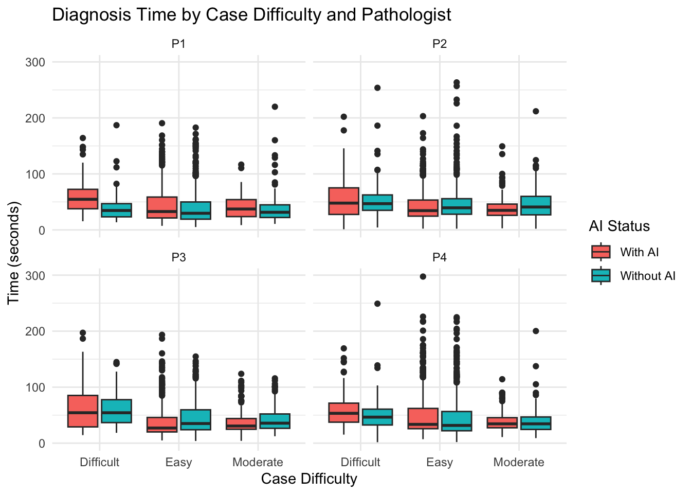
1 Difficult With AI P1 61.0 54.6 82
2 Difficult With AI P2 55.6 47.9 82
3 Difficult With AI P3 61.8 54.3 82
4 Difficult With AI P4 60.0 53.3 82
5 Difficult Without AI P1 40.4 34.7 82
6 Difficult Without AI P2 54.6 46.8 82
7 Difficult Without AI P3 60.3 54.3 82
8 Difficult Without AI P4 51.9 46.4 82
9 Easy With AI P1 44.4 32.8 570
10 Easy With AI P2 42.7 34.4 570
# ℹ 14 more rows# A tibble: 6 × 5
case_difficulty AI_status avg_time median_time sample_size
<chr> <chr> <dbl> <dbl> <int>
1 Difficult With AI 59.6 52.9 328
2 Difficult Without AI 51.8 44.2 328
3 Easy With AI 43.9 31.8 2280
4 Easy Without AI 43.9 34.1 2280
5 Moderate With AI 40.1 34.1 500
6 Moderate Without AI 42.1 34.8 500# A tibble: 3,108 × 7
Slide_Label Pathologist case_difficulty `Without AI` `With AI`
<chr> <chr> <chr> <dbl> <dbl>
1 c1_s2.svs P1 Moderate 84.9 69.9
2 c1_s2.svs P2 Moderate 33.4 26.0
3 c1_s2.svs P3 Moderate 35.3 56.7
4 c1_s2.svs P4 Moderate 58.7 37.5
5 c1_s3.svs P1 Easy 148. 80.8
6 c1_s3.svs P2 Easy 55.3 13.8
7 c1_s3.svs P3 Easy 21.2 46.6
8 c1_s3.svs P4 Easy 56.3 90.4
9 c1_s4.svs P1 Easy 155. 118.
10 c1_s4.svs P2 Easy 86.1 127.
# ℹ 3,098 more rows
# ℹ 2 more variables: time_difference <dbl>, percent_change <dbl># A tibble: 3 × 3
case_difficulty avg_time_difference avg_percent_change
<chr> <dbl> <dbl>
1 Difficult 7.82 57.8
2 Easy 0.0277 25.3
3 Moderate -2.02 23.6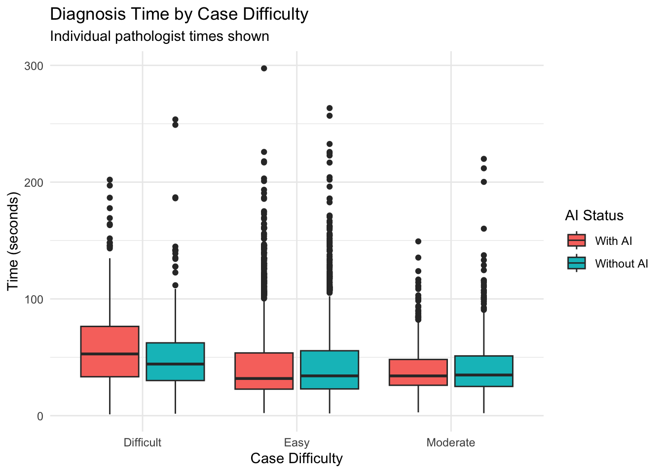
# A tibble: 8 × 5
  Pathologist changed_diagnosis avg_time median_time sample_size
  <chr>       <lgl>                <dbl>       <dbl>       <int>
1 P1          FALSE                 45.8        34.0         694
2 P1          TRUE                  44.7        39.6         129
3 P2          FALSE                 43.4        35.2         777
4 P2          TRUE                  46.8        35.5          46
5 P3          FALSE                 37.7        27.6         755
6 P3          TRUE                  73.6        75.0          68
7 P4          FALSE                 49.9        34.1         728
8 P4          TRUE                  50.1        43.8          95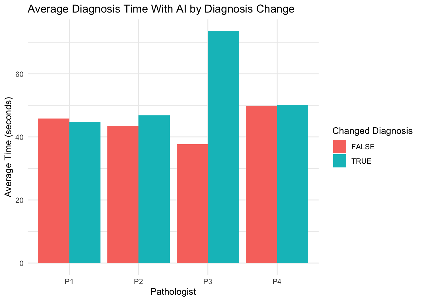
# A tibble: 6,248 × 153
   Slide_Label Dx_Paige Dx_Report Dx_Research Case_No.x Slide_No.x P1_noAI_Start
   <chr>       <chr>    <chr>     <chr>       <chr>          <dbl> <lgl>
 1 c1_s2.svs   Absent   Absent    Absent      c1                 2 TRUE
 2 c1_s2.svs   Absent   Absent    Absent      c1                 2 TRUE
 3 c1_s2.svs   Absent   Absent    Absent      c1                 2 TRUE
 4 c1_s2.svs   Absent   Absent    Absent      c1                 2 TRUE
 5 c1_s2.svs   Absent   Absent    Absent      c1                 2 TRUE
 6 c1_s2.svs   Absent   Absent    Absent      c1                 2 TRUE
 7 c1_s2.svs   Absent   Absent    Absent      c1                 2 TRUE
 8 c1_s2.svs   Absent   Absent    Absent      c1                 2 TRUE
 9 c1_s3.svs   Present  Present   Present     c1                 3 TRUE
10 c1_s3.svs   Present  Present   Present     c1                 3 TRUE
# ℹ 6,238 more rows
# ℹ 146 more variables: P1_noAI_Start_Time <dttm>, P1_noAI_Diagnosis <fct>,
#   P1_noAI_Primary <dbl>, P1_noAI_Secondary <dbl>, P1_noAI_PNI <chr>,
#   P1_noAI_Percent <chr>, P1_noAI_End <lgl>, P1_noAI_End_Time <dttm>,
#   P1_noAI_Comment <chr>, Case_No.y <chr>, Slide_No.y <dbl>,
#   P2_noAI_Start <lgl>, P2_noAI_Start_Time <dttm>, P2_noAI_Diagnosis <fct>,
#   P2_noAI_Primary <dbl>, P2_noAI_Secondary <dbl>, P2_noAI_PNI <chr>, …
# A tibble: 2 × 7
AI_status mean_time median_time min_time max_time sd_time n_observations
<chr> <dbl> <dbl> <dbl> <dbl> <dbl> <int>
1 With AI 44.8 33.7 1.16 297. 31.6 3124
2 Without AI 44.4 35.4 1.67 263. 30.8 3124# A tibble: 3,124 × 8
Slide_Label Pathologist `Without AI` `With AI` time_difference percent_change
<chr> <chr> <dbl> <dbl> <dbl> <dbl>
1 c1_s2.svs P1 84.9 69.9 -15.0 -17.6
2 c1_s2.svs P2 33.4 26.0 -7.36 -22.1
3 c1_s2.svs P3 35.3 56.7 21.4 60.7
4 c1_s2.svs P4 58.7 37.5 -21.2 -36.2
5 c1_s3.svs P1 148. 80.8 -67.1 -45.4
6 c1_s3.svs P2 55.3 13.8 -41.5 -75.1
7 c1_s3.svs P3 21.2 46.6 25.5 120.
8 c1_s3.svs P4 56.3 90.4 34.1 60.7
9 c1_s4.svs P1 155. 118. -36.4 -23.5
10 c1_s4.svs P2 86.1 127. 41.0 47.6
# ℹ 3,114 more rows
# ℹ 2 more variables: time_ratio <dbl>, is_faster <lgl># A tibble: 1 × 6
mean_diff median_diff mean_percent median_percent pct_faster n_cases
<dbl> <dbl> <dbl> <dbl> <dbl> <int>
1 0.456 0.522 28.2 1.78 48.7 3124
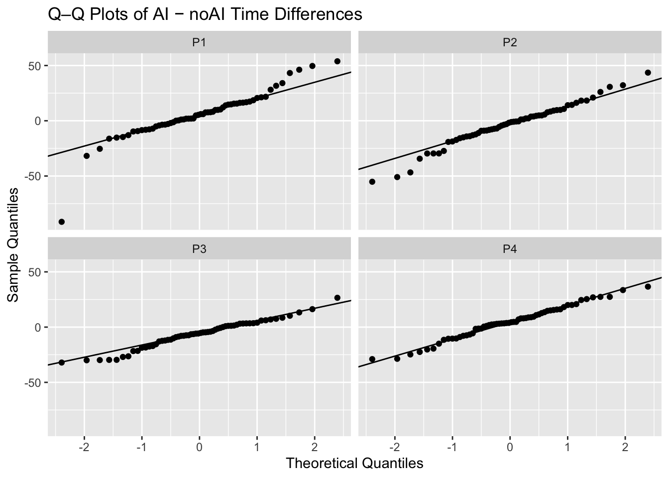
    Paired t-test

data:  time_diff_data$`With AI` and time_diff_data$`Without AI`
t = 0.77357, df = 3123, p-value = 0.4392
alternative hypothesis: true mean difference is not equal to 0
95 percent confidence interval:
 -0.699622  1.611398
sample estimates:
mean difference
0.455888 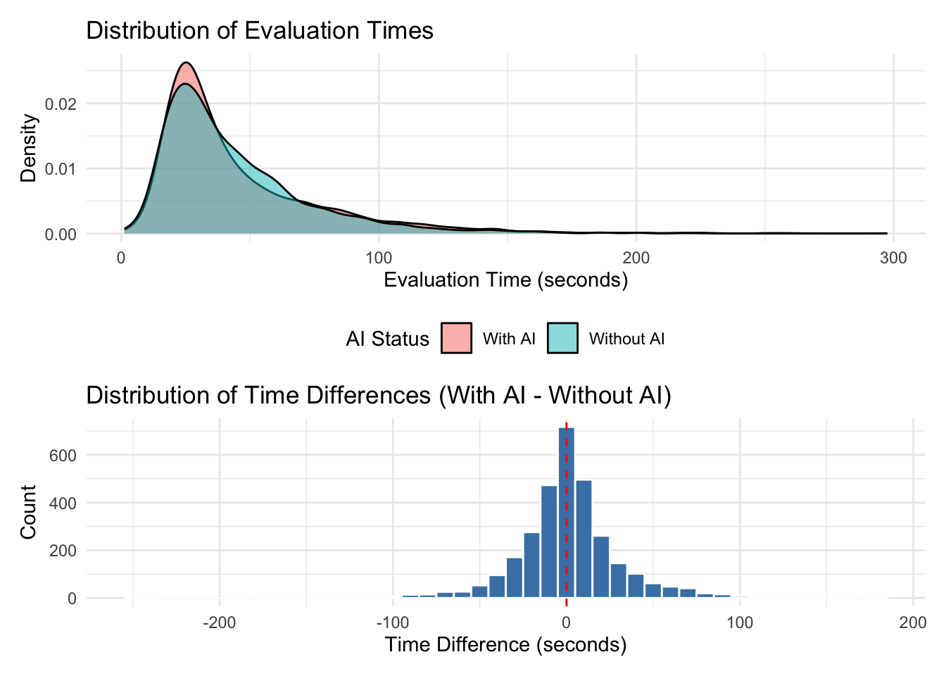
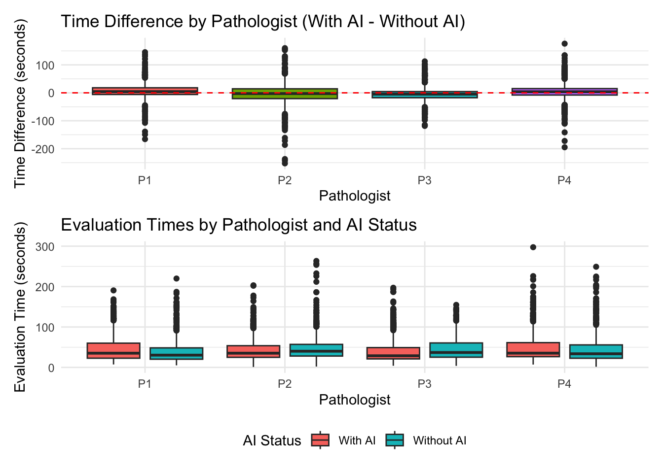
# A tibble: 8 × 6
  Pathologist AI         N  Mean Median    SD
  <chr>       <fct>  <int> <dbl>  <dbl> <dbl>
1 P1          noAI     781  39.3   30.4  28.6
2 P1          withAI   781  45.6   35.2  30.5
3 P2          noAI     781  46.9   40.1  30.7
4 P2          withAI   781  43.5   35.2  28.2
5 P3          noAI     781  46.0   36.9  27.5
6 P3          withAI   781  40.5   28.8  29.9
7 P4          noAI     781  45.4   33.7  35.3
8 P4          withAI   781  49.8   35.3  36.5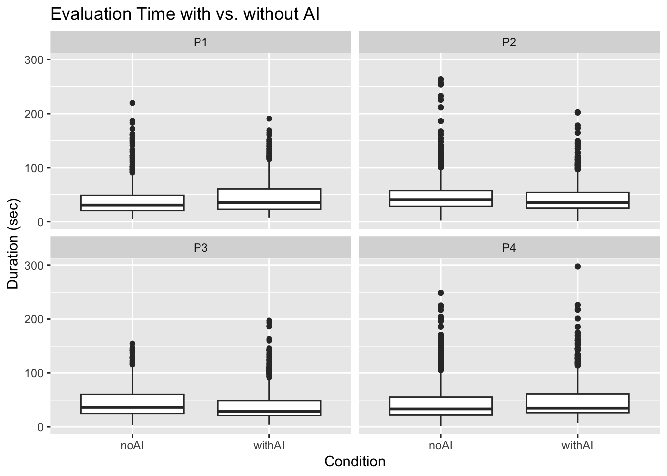
# A tibble: 480 × 4
   Case  Pathologist AI         n
   <chr> <chr>       <fct>  <int>
 1 c1    P1          noAI      12
 2 c1    P1          withAI    12
 3 c1    P2          noAI      12
 4 c1    P2          withAI    12
 5 c1    P3          noAI      12
 6 c1    P3          withAI    12
 7 c1    P4          noAI      12
 8 c1    P4          withAI    12
 9 c10   P1          noAI      12
10 c10   P1          withAI    12
# ℹ 470 more rows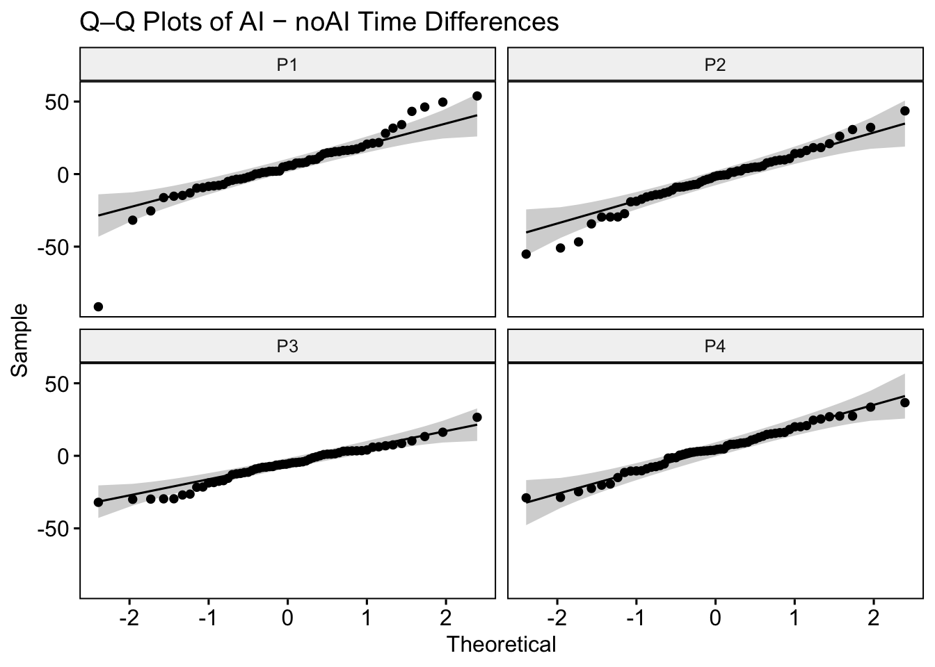
# A tibble: 4 × 4
  Pathologist t_stat    p_val mean_diff
  <chr>        <dbl>    <dbl>     <dbl>
1 P1            2.04 0.0459        5.59
2 P2           -1.40 0.165        -3.46
3 P3           -3.94 0.000215     -6.34
4 P4            2.27 0.0267        4.40
# A tibble: 4 × 3
Pathologist V_stat p_val
<chr> <dbl> <dbl>
1 P1 1281 0.00713
2 P2 759 0.252
3 P3 429 0.000351
4 P4 1234 0.0190 Linear mixed model fit by maximum likelihood . t-tests use Satterthwaite's
method [lmerModLmerTest]
Formula: Duration ~ AI + (1 | Case) + (1 | Pathologist)
Data: durations
AIC BIC logLik -2*log(L) df.resid
59142.7 59176.4 -29566.4 59132.7 6243
Scaled residuals:
Min 1Q Median 3Q Max
-2.8119 -0.5560 -0.1981 0.3331 8.4508
Random effects:
Groups Name Variance Std.Dev.
Case (Intercept) 260.41 16.137
Pathologist (Intercept) 4.51 2.124
Residual 728.14 26.984
Number of obs: 6248, groups: Case, 60; Pathologist, 4
Fixed effects:
Estimate Std. Error df t value Pr(>|t|)
(Intercept) 45.6162 2.3891 40.7743 19.093 <2e-16 ***
AIwithAI 0.4559 0.6828 6184.7648 0.668 0.504
---
Signif. codes: 0 '***' 0.001 '**' 0.01 '*' 0.05 '.' 0.1 ' ' 1
Correlation of Fixed Effects:
(Intr)
AIwithAI -0.143Type III Analysis of Variance Table with Satterthwaite's method
Sum Sq Mean Sq NumDF DenDF F value Pr(>F)
AI 324.64 324.64 1 6184.8 0.4458 0.5043# A tibble: 4 × 2
Pathologist d
<chr> <dbl>
1 P1 0.263
2 P2 -0.181
3 P3 -0.509
4 P4 0.293tibble [781 × 158] (S3: tbl_df/tbl/data.frame)
$ Slide_Label : chr [1:781] "c1_s2.svs" "c1_s3.svs" "c1_s4.svs" "c1_s5.svs" ...
$ Dx_Paige : chr [1:781] "Absent" "Present" "Present" "Present" ...
$ Dx_Report : chr [1:781] "Absent" "Present" "Present" "Present" ...
$ Dx_Research : chr [1:781] "Absent" "Present" "Present" "Present" ...
$ Case_No.x : chr [1:781] "c1" "c1" "c1" "c1" ...
$ Slide_No.x : num [1:781] 2 3 4 5 6 7 8 9 10 11 ...
$ P1_noAI_Start : logi [1:781] TRUE TRUE TRUE TRUE TRUE TRUE ...
$ P1_noAI_Start_Time : POSIXct[1:781], format: "2023-04-26 14:00:55" "2023-04-26 14:02:33" ...
$ P1_noAI_Diagnosis : chr [1:781] "Malignant" "Malignant" "Malignant" "Malignant" ...
$ P1_noAI_Primary : num [1:781] 4 4 3 3 3 NA NA NA NA NA ...
$ P1_noAI_Secondary : num [1:781] 4 3 4 4 4 NA NA NA NA NA ...
$ P1_noAI_PNI : chr [1:781] "Negative" "Negative" "Positive" "Negative" ...
$ P1_noAI_Percent : chr [1:781] "45056.0" "45056.0" "60-70" "70-80" ...
$ P1_noAI_End : logi [1:781] TRUE TRUE TRUE TRUE TRUE TRUE ...
$ P1_noAI_End_Time : POSIXct[1:781], format: "2023-04-26 14:02:20" "2023-04-26 14:05:01" ...
$ P1_noAI_Comment : logi [1:781] NA NA NA NA NA NA ...
$ Case_No.y : chr [1:781] "c1" "c1" "c1" "c1" ...
$ Slide_No.y : num [1:781] 2 3 4 5 6 7 8 9 10 11 ...
$ P2_noAI_Start : logi [1:781] TRUE TRUE TRUE TRUE TRUE TRUE ...
$ P2_noAI_Start_Time : POSIXct[1:781], format: "2023-04-25 14:39:17" "2023-04-25 14:39:52" ...
$ P2_noAI_Diagnosis : chr [1:781] "Malignant" "Malignant" "Malignant" "Malignant" ...
$ P2_noAI_Primary : num [1:781] 4 4 4 4 4 NA NA NA NA NA ...
$ P2_noAI_Secondary : num [1:781] 3 3 3 3 3 NA NA NA NA NA ...
$ P2_noAI_PNI : chr [1:781] "Negative" "Negative" "Negative" "Negative" ...
$ P2_noAI_Percent : chr [1:781] "45056.0" "40-50" "50-60" "60-70" ...
$ P2_noAI_End : logi [1:781] TRUE TRUE TRUE TRUE TRUE TRUE ...
$ P2_noAI_End_Time : POSIXct[1:781], format: "2023-04-25 14:39:50" "2023-04-25 14:40:47" ...
$ P2_noAI_Comment : logi [1:781] NA NA NA NA NA NA ...
$ Case_No.x.x : chr [1:781] "c1" "c1" "c1" "c1" ...
$ Slide_No.x.x : num [1:781] 2 3 4 5 6 7 8 9 10 11 ...
$ P3_noAI_Start : logi [1:781] TRUE TRUE TRUE TRUE TRUE TRUE ...
$ P3_noAI_Start_Time : POSIXct[1:781], format: "2023-06-14 10:09:19" "2023-06-14 10:18:55" ...
$ P3_noAI_Diagnosis : chr [1:781] "IHC" "Malignant" "Malignant" "Malignant" ...
$ P3_noAI_Primary : num [1:781] 4 4 4 4 4 NA NA NA NA NA ...
$ P3_noAI_Secondary : num [1:781] 4 4 4 3 4 NA NA NA NA NA ...
$ P3_noAI_PNI : chr [1:781] "Negative" "Negative" "Negative" "Negative" ...
$ P3_noAI_Percent : chr [1:781] "45056.0" "0-5" "50-60" "80-90" ...
$ P3_noAI_End : logi [1:781] TRUE TRUE TRUE TRUE TRUE TRUE ...
$ P3_noAI_End_Time : POSIXct[1:781], format: "2023-06-14 10:09:54" "2023-06-14 10:19:17" ...
$ P3_noAI_Comment : chr [1:781] NA NA NA NA ...
$ Case_No.y.y : chr [1:781] "c1" "c1" "c1" "c1" ...
$ Slide_No.y.y : num [1:781] 2 3 4 5 6 7 8 9 10 11 ...
$ P4_noAI_Start : num [1:781] 1 1 1 1 1 1 1 1 1 1 ...
$ P4_noAI_Start_Time : POSIXct[1:781], format: "2023-05-13 12:42:56" "2023-05-13 12:45:14" ...
$ P4_noAI_Diagnosis : chr [1:781] "Malignant" "Malignant" "Malignant" "Malignant" ...
$ P4_noAI_Primary : num [1:781] 4 4 4 4 4 NA NA NA NA NA ...
$ P4_noAI_Secondary : num [1:781] 4 4 3 4 4 NA NA NA NA NA ...
$ P4_noAI_PNI : chr [1:781] "Negative" "Negative" "Positive" "Negative" ...
$ P4_noAI_Percent : chr [1:781] "45219.0" "45219.0" "80-90" "80-90" ...
$ P4_noAI_End : num [1:781] 1 1 1 1 1 1 1 1 1 1 ...
$ P4_noAI_End_Time : POSIXct[1:781], format: "2023-05-13 12:43:55" "2023-05-13 12:46:10" ...
$ P4_noAI_Comment : chr [1:781] NA NA NA NA ...
$ Case_No.x.x.x : chr [1:781] "c1" "c1" "c1" "c1" ...
$ Slide_No.x.x.x : num [1:781] 2 3 4 5 6 7 8 9 10 11 ...
$ P1_withAI_Start : logi [1:781] TRUE TRUE TRUE TRUE TRUE TRUE ...
$ P1_withAI_Start_Time : POSIXct[1:781], format: "2023-07-06 10:53:41" "2023-07-06 11:00:00" ...
$ P1_withAI_Diagnosis : chr [1:781] "Consult" "Malignant" "Malignant" "Malignant" ...
$ P1_withAI_Primary : num [1:781] NA 4 3 3 3 NA NA NA NA NA ...
$ P1_withAI_Secondary : num [1:781] NA 4 4 4 4 NA NA NA NA NA ...
$ P1_withAI_PNI : chr [1:781] NA "Negative" "Positive" "Negative" ...
$ P1_withAI_Percent : chr [1:781] NA "40-50" "70-80" "80-90" ...
$ P1_withAI_End : logi [1:781] TRUE TRUE TRUE TRUE TRUE TRUE ...
$ P1_withAI_End_Time : POSIXct[1:781], format: "2023-07-06 10:54:51" "2023-07-06 11:01:21" ...
$ P1_withAI_AIHelpful : chr [1:781] "AI tanı vermeme engel oldu" "AI gereksizdi" "AI gereksizdi" "AI gereksizdi" ...
$ P1_withAI_AIAgree : chr [1:781] "AI tanısına katılmadım" "AI tanısına katılmadım" "AI tanısına katıldım" "AI tanısına katıldım" ...
$ P1_withAI_Comment : chr [1:781] "yeni kesit görmek isterdim. konsülte etmek istediğim bir odak var." "PNI için işaretlediği alana katılmadım. Bulanık bir alan." "PNI AI'da değerlendirilmemiş." "PNI AI'da değerlendirilmemiş." ...
$ Case_No.y.y.y : chr [1:781] "c1" "c1" "c1" "c1" ...
$ Slide_No.y.y.y : num [1:781] 2 3 4 5 6 7 8 9 10 11 ...
$ P2_withAI_Start : logi [1:781] TRUE TRUE TRUE TRUE TRUE TRUE ...
$ P2_withAI_Start_Time : POSIXct[1:781], format: "2023-09-07 16:21:55" "2023-09-07 16:22:24" ...
$ P2_withAI_Diagnosis : chr [1:781] "Malignant" "Malignant" "Malignant" "Malignant" ...
$ P2_withAI_Primary : num [1:781] 4 4 4 4 4 NA NA NA NA NA ...
$ P2_withAI_Secondary : num [1:781] 3 4 3 3 3 NA NA NA NA NA ...
$ P2_withAI_PNI : chr [1:781] "Negative" "Negative" "Positive" "Negative" ...
$ P2_withAI_Percent : chr [1:781] "45056" "40-50" "60-70" "70-80" ...
$ P2_withAI_End : logi [1:781] TRUE TRUE TRUE TRUE TRUE TRUE ...
$ P2_withAI_End_Time : POSIXct[1:781], format: "2023-09-07 16:22:21" "2023-09-07 16:22:37" ...
$ P2_withAI_AIHelpful : chr [1:781] "AI gereksizdi" "AI tanıya yardımcı oldu" "AI tanıya yardımcı oldu" "AI tanıya yardımcı oldu" ...
$ P2_withAI_AIAgree : chr [1:781] "AI tümörü atlamış" "AI tanısına katıldım" "AI tanısına katıldım" "AI tanısına katıldım" ...
$ P2_withAI_Comment : chr [1:781] NA NA "perinöralı değerlendirmemiş" NA ...
$ Case_No.x.x.x.x : chr [1:781] "c1" "c1" "c1" "c1" ...
$ Slide_No.x.x.x.x : num [1:781] 2 3 4 5 6 7 8 9 10 11 ...
$ P3_withAI_Start : logi [1:781] TRUE TRUE TRUE TRUE TRUE TRUE ...
$ P3_withAI_Start_Time : POSIXct[1:781], format: "2023-09-08 16:30:41" "2023-09-08 16:33:09" ...
$ P3_withAI_Diagnosis : chr [1:781] "IHC" "Malignant" "Malignant" "Malignant" ...
$ P3_withAI_Primary : num [1:781] NA 4 3 3 3 NA NA NA NA NA ...
$ P3_withAI_Secondary : num [1:781] NA 4 4 4 4 NA NA NA NA NA ...
$ P3_withAI_PNI : chr [1:781] "Negative" "Negative" "Negative" "Negative" ...
$ P3_withAI_Percent : chr [1:781] "45056.0" "40-50" "70-80" "70-80" ...
$ P3_withAI_End : logi [1:781] TRUE TRUE TRUE TRUE TRUE TRUE ...
$ P3_withAI_End_Time : POSIXct[1:781], format: "2023-09-08 16:31:38" "2023-09-08 16:33:56" ...
$ P3_withAI_AIHelpful : chr [1:781] NA "AI tanıya yardımcı oldu" "AI tanıya yardımcı oldu" "AI tanıya yardımcı oldu" ...
$ P3_withAI_AIAgree : chr [1:781] NA "AI tanısına katıldım" "AI tanısına katıldım" "AI tanısına katıldım" ...
$ P3_withAI_Comment : chr [1:781] "AI yok" NA NA NA ...
$ Case_No.y.y.y.y : chr [1:781] "c1" "c1" "c1" "c1" ...
$ Slide_No.y.y.y.y : num [1:781] 2 3 4 5 6 7 8 9 10 11 ...
$ P4_withAI_Start : logi [1:781] TRUE TRUE TRUE TRUE TRUE TRUE ...
$ P4_withAI_Start_Time : POSIXct[1:781], format: "2023-08-20 20:00:40" "2023-08-20 20:02:01" ...
$ P4_withAI_Diagnosis : chr [1:781] "Malignant" "Malignant" "Malignant" "Malignant" ...
[list output truncated] P1_noAI_interval_seconds P2_noAI_interval_seconds P3_noAI_interval_seconds
Min. : 5.08 Min. : 2.152 Min. : 3.857
1st Qu.: 20.32 1st Qu.: 28.110 1st Qu.: 25.273
Median : 30.37 Median : 40.113 Median : 36.892
Mean : 39.27 Mean : 46.872 Mean : 45.976
3rd Qu.: 48.30 3rd Qu.: 56.994 3rd Qu.: 60.519
Max. :219.94 Max. :263.427 Max. :154.722
P4_noAI_interval_seconds P1_withAI_interval_seconds P2_withAI_interval_seconds
Min. : 1.669 Min. : 7.275 Min. : 1.164
1st Qu.: 22.712 1st Qu.: 22.766 1st Qu.: 24.960
Median : 33.741 Median : 35.186 Median : 35.195
Mean : 45.419 Mean : 45.555 Mean : 43.537
3rd Qu.: 55.701 3rd Qu.: 60.000 3rd Qu.: 53.707
Max. :249.057 Max. :190.567 Max. :203.142
P3_withAI_interval_seconds P4_withAI_interval_seconds
Min. : 4.067 Min. : 7.048
1st Qu.: 21.040 1st Qu.: 26.580
Median : 28.773 Median : 35.277
Mean : 40.484 Mean : 49.781
3rd Qu.: 49.002 3rd Qu.: 61.283
Max. :197.134 Max. :297.455 # A tibble: 2 × 7
ai_status mean_time median_time min_time max_time sd_time n_observations
<chr> <dbl> <dbl> <dbl> <dbl> <dbl> <int>
1 With AI 44.8 33.7 1.16 297. 31.6 3124
2 Without AI 44.4 35.4 1.67 263. 30.8 3124# A tibble: 1 × 6
mean_diff_seconds median_diff_seconds mean_percent_change
<dbl> <dbl> <dbl>
1 0.456 0.522 28.2
# ℹ 3 more variables: median_percent_change <dbl>, pct_cases_faster <dbl>,
# n_cases <int>
    Paired t-test

data:  time_differences$`With AI` and time_differences$`Without AI`
t = 0.77357, df = 3123, p-value = 0.4392
alternative hypothesis: true mean difference is not equal to 0
95 percent confidence interval:
 -0.699622  1.611398
sample estimates:
mean difference
0.455888 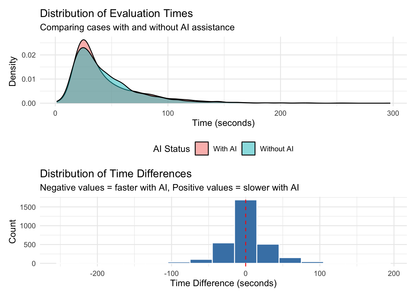
# A tibble: 4 × 6
  pathologist mean_diff median_diff mean_percent pct_faster n_cases
  <chr>           <dbl>       <dbl>        <dbl>      <dbl>   <int>
1 P1               6.29        4.24        38.4        38.5     781
2 P2              -3.33       -2.72        39.4        55.2     781
3 P3              -5.49       -4.65        -1.32       62.1     781
4 P4               4.36        3.92        36.5        39.1     781
Df Sum Sq Mean Sq F value Pr(>F)
pathologist 3 77329 25776 24.29 1.56e-15 ***
Residuals 3120 3311094 1061
---
Signif. codes: 0 '***' 0.001 '**' 0.01 '*' 0.05 '.' 0.1 ' ' 1 Tukey multiple comparisons of means
95% family-wise confidence level
Fit: aov(formula = time_difference ~ pathologist, data = time_differences)
$pathologist
diff lwr upr p adj
P2-P1 -9.622565 -13.859984 -5.385145 0.0000000
P3-P1 -11.779119 -16.016538 -7.541700 0.0000000
P4-P1 -1.925151 -6.162570 2.312268 0.6472736
P3-P2 -2.156554 -6.393974 2.080865 0.5577439
P4-P2 7.697414 3.459994 11.934833 0.0000187
P4-P3 9.853968 5.616549 14.091387 0.0000000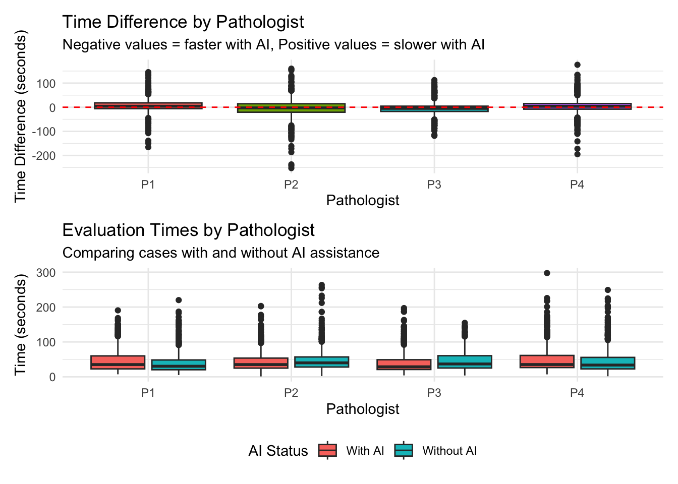
# A tibble: 4 × 6
  case_difficulty mean_diff median_diff mean_percent pct_faster n_cases
  <chr>               <dbl>       <dbl>        <dbl>      <dbl>   <int>
1 Difficult          7.82         6.41          57.8       41.8     328
2 Easy               0.0277       0.491         25.3       48.6    2280
3 Moderate          -2.02        -1.26          23.6       53       500
4 <NA>             -11.9         -9.32         -15.8       75        16
Df Sum Sq Mean Sq F value Pr(>F)
case_difficulty 2 21251 10626 9.826 5.57e-05 ***
Residuals 3105 3357665 1081
---
Signif. codes: 0 '***' 0.001 '**' 0.01 '*' 0.05 '.' 0.1 ' ' 1
16 observations deleted due to missingness Tukey multiple comparisons of means
95% family-wise confidence level
Fit: aov(formula = time_difference ~ case_difficulty, data = time_diff_with_context)
$case_difficulty
diff lwr upr p adj
Easy-Difficult -7.788601 -12.342131 -3.235072 0.0001830
Moderate-Difficult -9.840900 -15.319782 -4.362017 0.0000773
Moderate-Easy -2.052298 -5.860051 1.755454 0.4158488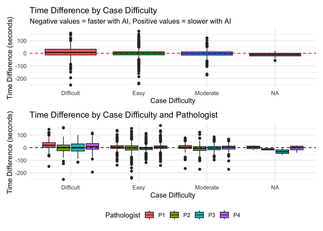
# A tibble: 3 × 6
  diagnosis_changed mean_diff median_diff mean_percent pct_faster n_cases
  <lgl>                 <dbl>       <dbl>        <dbl>      <dbl>   <int>
1 FALSE                 0.395       0.528         26.0       48.5    2806
2 TRUE                  1.11        0.205         48.5       50       314
3 NA                   -8.83       -6.55         -11.2       75         4
    Welch Two Sample t-test

data:  time_difference by diagnosis_changed
t = -0.25917, df = 342.33, p-value = 0.7957
alternative hypothesis: true difference in means between group FALSE and group TRUE is not equal to 0
95 percent confidence interval:
 -6.178803  4.740101
sample estimates:
mean in group FALSE  mean in group TRUE
0.3953913 1.1147420 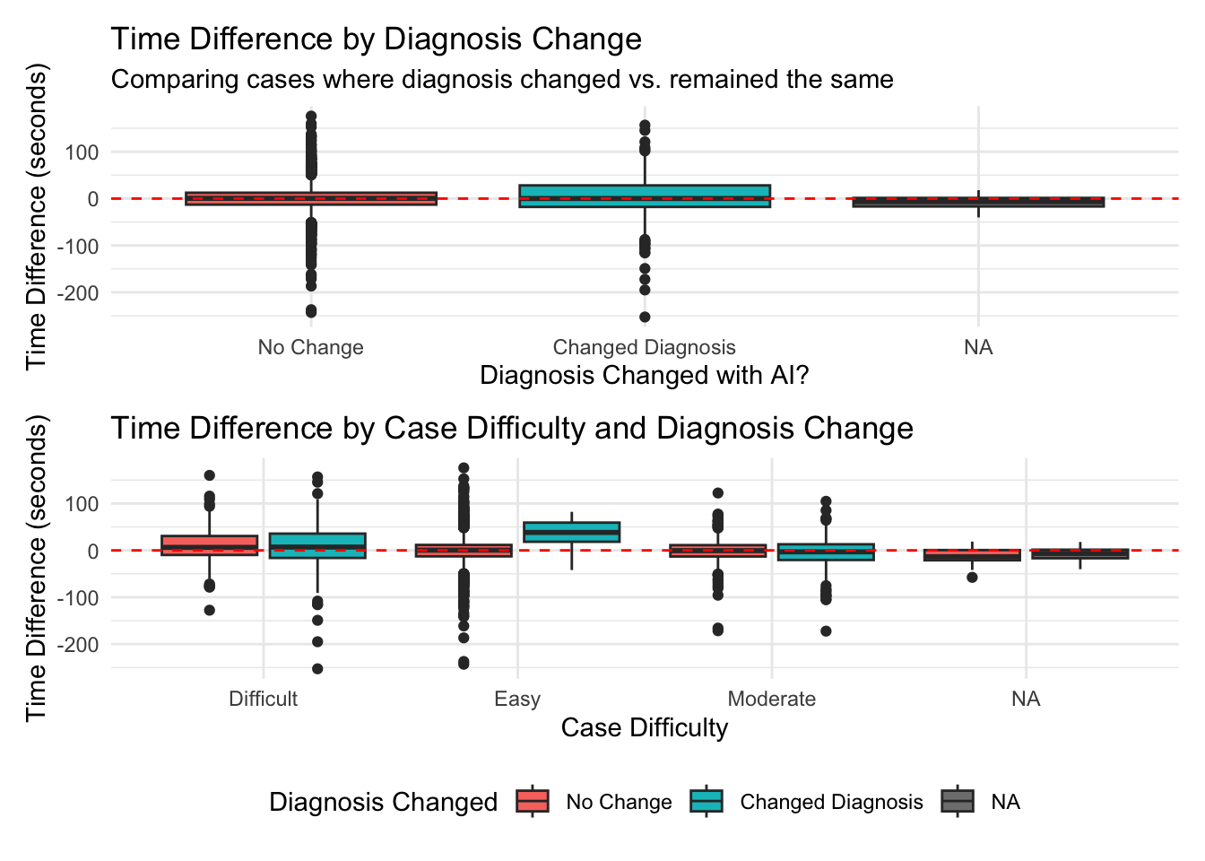
# A tibble: 4 × 6
  Transition_Type mean_diff median_diff mean_percent pct_faster n_cases
  <chr>               <dbl>       <dbl>        <dbl>      <dbl>   <int>
1 Improvement        -1.38       -1.49          24.7       53.3     644
2 No Change           0.550       0.824         27.6       47.7    2380
3 Worsening          14.2        11.2           80.8       38.1      84
4 <NA>              -11.9        -9.32         -15.8       75        16
Df Sum Sq Mean Sq F value Pr(>F)
Transition_Type 2 18033 9017 8.33 0.000247 ***
Residuals 3105 3360883 1082
---
Signif. codes: 0 '***' 0.001 '**' 0.01 '*' 0.05 '.' 0.1 ' ' 1
16 observations deleted due to missingness Tukey multiple comparisons of means
95% family-wise confidence level
Fit: aov(formula = time_difference ~ Transition_Type, data = time_with_agreement)
$Transition_Type
diff lwr upr p adj
No Change-Improvement 1.925686 -1.500937 5.352308 0.3853433
Worsening-Improvement 15.574412 6.625096 24.523728 0.0001362
Worsening-No Change 13.648726 5.084286 22.213166 0.0005560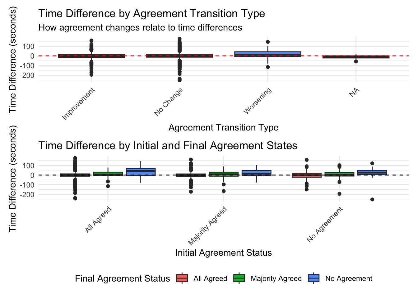
# A tibble: 3 × 6
  ai_helpful               mean_diff median_diff mean_percent pct_faster n_cases
  <chr>                        <dbl>       <dbl>        <dbl>      <dbl>   <int>
1 AI gereksizdi                 2.52        1.79         26.3       44.7    1842
2 AI tanı vermeme engel o…     13.6        19.0          80.6       25.9      81
3 AI tanıya yardımcı oldu      -3.64       -3.48         27.6       56.5    1195
# A tibble: 4 × 6
ai_agree mean_diff median_diff mean_percent pct_faster n_cases
<chr> <dbl> <dbl> <dbl> <dbl> <int>
1 AI gereksiz şüphe koydu 23.2 24.2 103. 19.6 46
2 AI tanısına katıldım -1.11 -0.291 24.3 50.6 2886
3 AI tanısına katılmadım 18.3 20.3 70.5 27.3 176
4 AI tümörü atlamış 26.7 21.7 68.2 25 8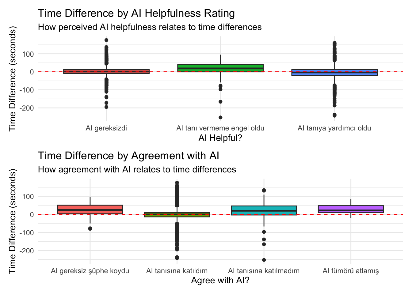
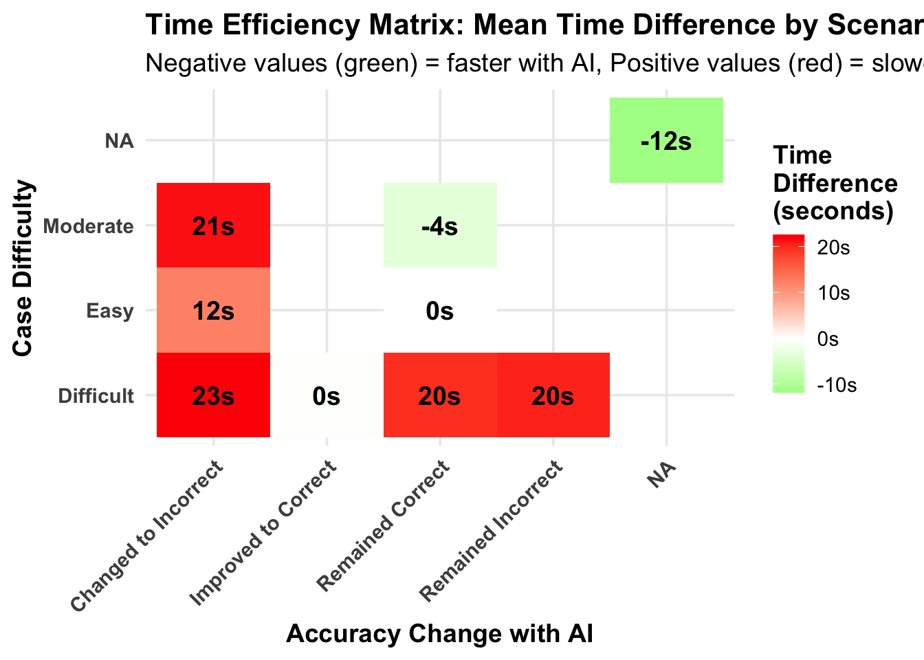
# A tibble: 5 × 6
  accuracy_change      mean_diff median_diff mean_percent pct_faster n_cases
  <chr>                    <dbl>       <dbl>        <dbl>      <dbl>   <int>
1 Changed to Incorrect    21.3        18.6           89.0       31.2      64
2 Improved to Correct     -0.334       0.754         38.0       49       200
3 Remained Correct        -0.207       0.291         25.0       49.4    2800
4 Remained Incorrect      20.4        24.5          118.        22.7      44
5 <NA>                   -11.9        -9.32         -15.8       75        16
Df Sum Sq Mean Sq F value Pr(>F)
accuracy_change 3 46653 15551 14.49 2.27e-09 ***
Residuals 3104 3332264 1074
---
Signif. codes: 0 '***' 0.001 '**' 0.01 '*' 0.05 '.' 0.1 ' ' 1
16 observations deleted due to missingness Tukey multiple comparisons of means
95% family-wise confidence level
Fit: aov(formula = time_difference ~ accuracy_change, data = time_with_accuracy)
$accuracy_change
diff lwr upr
Improved to Correct-Changed to Incorrect -21.6192506 -33.714380 -9.524121
Remained Correct-Changed to Incorrect -21.4919717 -32.139065 -10.844879
Remained Incorrect-Changed to Incorrect -0.8611520 -17.354511 15.632207
Remained Correct-Improved to Correct 0.1272789 -6.036970 6.291528
Remained Incorrect-Improved to Correct 20.7580987 6.734253 34.781944
Remained Incorrect-Remained Correct 20.6308197 7.834856 33.426783
p adj
Improved to Correct-Changed to Incorrect 0.0000267
Remained Correct-Changed to Incorrect 0.0000013
Remained Incorrect-Changed to Incorrect 0.9991374
Remained Correct-Improved to Correct 0.9999463
Remained Incorrect-Improved to Correct 0.0008331
Remained Incorrect-Remained Correct 0.0002049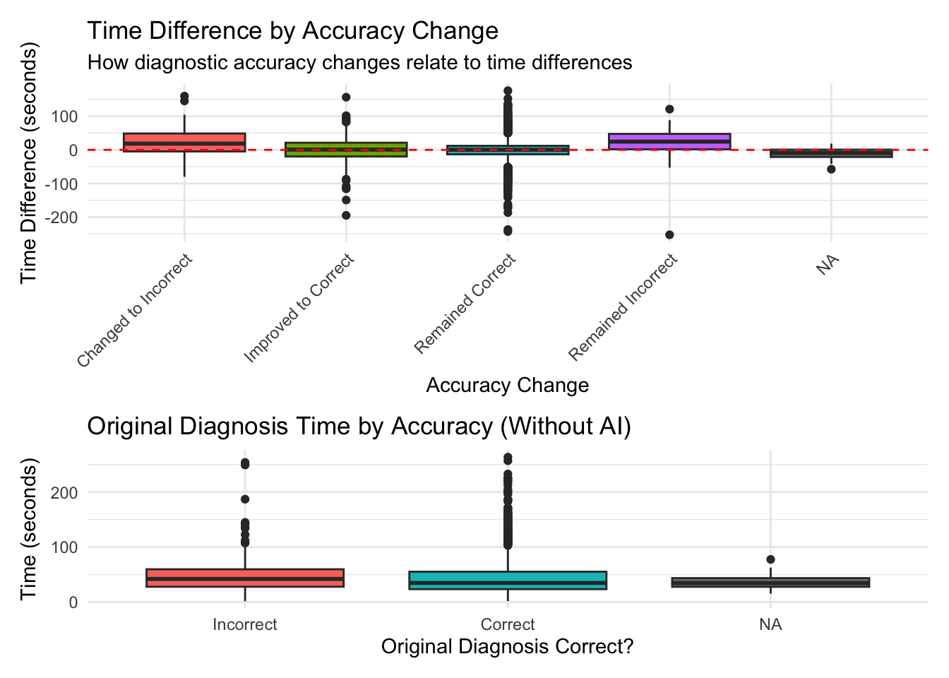
Linear mixed model fit by REML. t-tests use Satterthwaite's method [
lmerModLmerTest]
Formula:
time_difference ~ case_difficulty + diagnosis_changed + Transition_Type +
    accuracy_change + (1 | pathologist)
   Data: modeling_data

REML criterion at convergence: 30378.5

Scaled residuals:
    Min      1Q  Median      3Q     Max
-8.2140 -0.4037  0.0111  0.3827  5.3383

Random effects:
 Groups      Name        Variance Std.Dev.
 pathologist (Intercept)   34.12   5.841
 Residual                1040.15  32.251
Number of obs: 3108, groups:  pathologist, 4

Fixed effects:
                                   Estimate Std. Error       df t value
(Intercept)                          27.706      6.590   70.830   4.204
case_difficultyEasy                 -24.574      4.964 3096.291  -4.950
case_difficultyModerate             -19.483      4.018 3096.035  -4.849
diagnosis_changedTRUE                -6.480      2.369 3098.945  -2.735
Transition_TypeNo Change              7.569      3.526 3096.018   2.147
Transition_TypeWorsening             10.795      5.095 3096.060   2.119
accuracy_changeImproved to Correct  -25.383      6.085 3096.001  -4.172
accuracy_changeRemained Correct     -10.709      5.791 3095.998  -1.849
accuracy_changeRemained Incorrect   -12.494      7.831 3096.009  -1.595
                                   Pr(>|t|)
(Intercept)                        7.53e-05 ***
case_difficultyEasy                7.81e-07 ***
case_difficultyModerate            1.30e-06 ***
diagnosis_changedTRUE               0.00626 **
Transition_TypeNo Change            0.03191 *
Transition_TypeWorsening            0.03418 *
accuracy_changeImproved to Correct 3.11e-05 ***
accuracy_changeRemained Correct     0.06451 .
accuracy_changeRemained Incorrect   0.11071
---
Signif. codes:  0 '***' 0.001 '**' 0.01 '*' 0.05 '.' 0.1 ' ' 1

Correlation of Fixed Effects:
            (Intr) cs_dfE cs_dfM d_TRUE Tr_TNC Trn_TW ac_ItC acc_RC
cs_dffcltyE -0.136
cs_dffcltyM -0.306  0.724
dgnss_cTRUE -0.154  0.241  0.085
Trnstn_TyNC -0.178 -0.586  0.016 -0.062
Trnstn_TypW -0.521 -0.301 -0.083 -0.110  0.365
accrcy_cItC -0.814  0.115  0.319 -0.027  0.187  0.535
accrcy_chRC -0.686 -0.331 -0.282  0.006  0.099  0.622  0.711
accrcy_chRI -0.579  0.352  0.241  0.047 -0.294  0.286  0.604  0.532
Analysis of Deviance Table (Type II Wald chisquare tests)
Response: time_difference
Chisq Df Pr(>Chisq)
case_difficulty 27.8626 2 8.906e-07 ***
diagnosis_changed 7.4827 1 0.0062293 **
Transition_Type 6.6652 2 0.0356999 *
accuracy_change 20.6878 3 0.0001222 ***
---
Signif. codes: 0 '***' 0.001 '**' 0.01 '*' 0.05 '.' 0.1 ' ' 1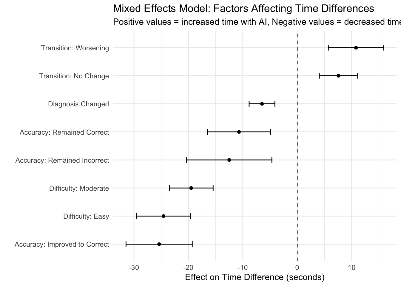
                                   Metric                            Value
1                Overall Mean Time Change                0 seconds (28.2%)
2              Overall Median Time Change                 1 seconds (1.8%)
3         Percent of Cases Faster with AI                            48.7%
4    Pathologist with Most Time Reduction                               P3
5  Case Difficulty with Most Time Benefit                             <NA>
6     Scenario with Greatest Time Savings                          NA & NA
7    Scenario with Greatest Time Increase Difficult & Changed to Incorrect
8 Statistical Significance of Time Change      Not significant (p = 0.439)
9    Most Important Factor in Time Change    Accuracy: Improved to Correct
Time Efficiency and Learning Effects Analysis for Pathologist Evaluation Time with AI
I’ll add a comprehensive analysis of time efficiency patterns and potential learning effects to understand whether pathologists become more efficient with AI assistance over time. This analysis will help determine if there’s a pattern of increasing time savings as pathologists gain experience with AI.
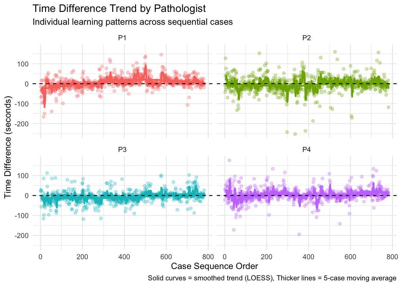
  Pathologist Correlation      P_Value Significant
1     Overall   0.2380957 1.627604e-41        TRUE
2          P1   0.3568894 0.000000e+00        TRUE
3          P2   0.1524802 1.915957e-05        TRUE
4          P3   0.3160171 1.425390e-19        TRUE
5          P4   0.1635390 4.349025e-06        TRUE
# A tibble: 3,124 × 13
pathologist Slide_Label `Without AI` `With AI` time_difference percent_change
<chr> <chr> <dbl> <dbl> <dbl> <dbl>
1 P1 c1_s2.svs 84.9 69.9 -15.0 -17.6
2 P1 c1_s3.svs 148. 80.8 -67.1 -45.4
3 P1 c1_s4.svs 155. 118. -36.4 -23.5
4 P1 c1_s5.svs 39.3 55.0 15.7 39.9
5 P1 c1_s6.svs 80.7 45.6 -35.2 -43.6
6 P1 c1_s7.svs 82.8 18.3 -64.4 -77.9
7 P1 c1_s8.svs 57.0 28.0 -29.0 -50.9
8 P1 c1_s9.svs 116. 20.2 -95.9 -82.6
9 P1 c1_s10.svs 41.5 18.4 -23.1 -55.7
10 P1 c1_s11.svs 45.2 24.5 -20.7 -45.8
# ℹ 3,114 more rows
# ℹ 7 more variables: is_faster <lgl>, P1_case_order <int>,
# P2_case_order <int>, P3_case_order <int>, P4_case_order <int>,
# case_order <dbl>, moving_avg <dbl>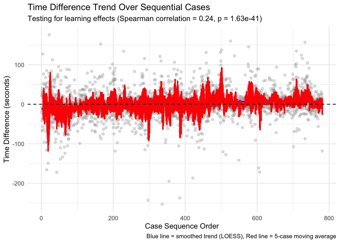
# A tibble: 3,124 × 13
   Slide_Label pathologist `Without AI` `With AI` time_difference percent_change
   <chr>       <chr>              <dbl>     <dbl>           <dbl>          <dbl>
 1 c1_s2.svs   P1                  84.9      69.9          -15.0           -17.6
 2 c1_s2.svs   P2                  33.4      26.0           -7.36          -22.1
 3 c1_s2.svs   P3                  35.3      56.7           21.4            60.7
 4 c1_s2.svs   P4                  58.7      37.5          -21.2           -36.2
 5 c1_s3.svs   P1                 148.       80.8          -67.1           -45.4
 6 c1_s3.svs   P2                  55.3      13.8          -41.5           -75.1
 7 c1_s3.svs   P3                  21.2      46.6           25.5           120.
 8 c1_s3.svs   P4                  56.3      90.4           34.1            60.7
 9 c1_s4.svs   P1                 155.      118.           -36.4           -23.5
10 c1_s4.svs   P2                  86.1     127.            41.0            47.6
# ℹ 3,114 more rows
# ℹ 7 more variables: is_faster <lgl>, P1_case_order <int>,
#   P2_case_order <int>, P3_case_order <int>, P4_case_order <int>,
#   case_order <dbl>, case_difficulty <chr>
# A tibble: 3,124 × 14
pathologist case_difficulty Slide_Label `Without AI` `With AI`
<chr> <chr> <chr> <dbl> <dbl>
1 P1 Difficult c2_s2.svs 43.0 24.3
2 P1 Difficult c2_s7.svs 187. 37.9
3 P1 Difficult c4_s3.svs 73.6 27.6
4 P1 Difficult c4_s14.svs 58.5 16.8
5 P1 Difficult c5_s1.svs 123. 135.
6 P1 Difficult c6_s7.svs 30.4 20.5
7 P1 Difficult c6_s8.svs 58.4 23.5
8 P1 Difficult c6_s10.svs 36.6 29.9
9 P1 Difficult c7_s3.svs 55.9 97.5
10 P1 Difficult c7_s7.svs 43.9 87.0
# ℹ 3,114 more rows
# ℹ 9 more variables: time_difference <dbl>, percent_change <dbl>,
# is_faster <lgl>, P1_case_order <int>, P2_case_order <int>,
# P3_case_order <int>, P4_case_order <int>, case_order <dbl>,
# moving_avg <dbl>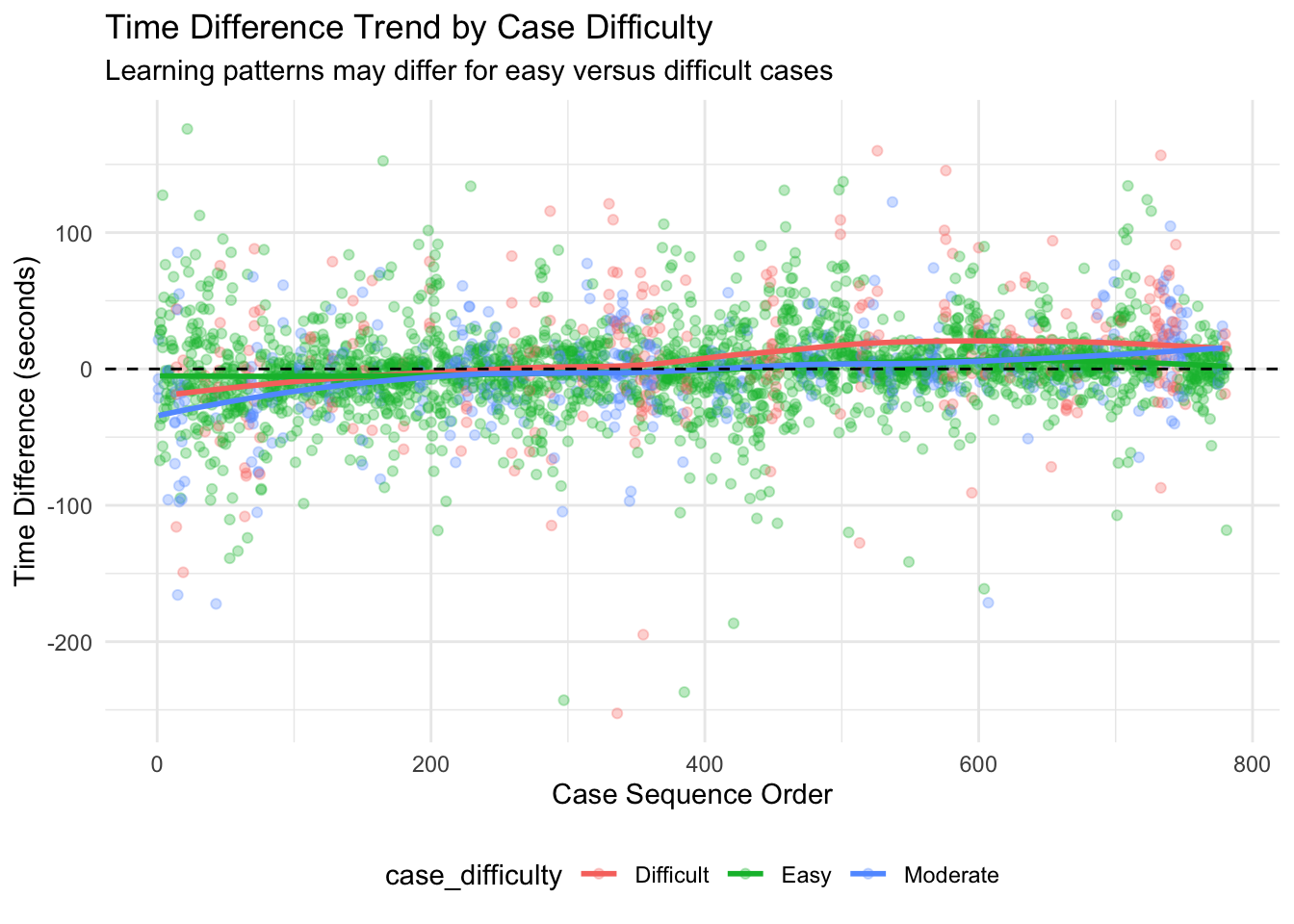
# A tibble: 3,124 × 14
   Slide_Label pathologist `Without AI` `With AI` time_difference percent_change
   <chr>       <chr>              <dbl>     <dbl>           <dbl>          <dbl>
 1 c1_s2.svs   P1                  84.9      69.9          -15.0           -17.6
 2 c1_s2.svs   P2                  33.4      26.0           -7.36          -22.1
 3 c1_s2.svs   P3                  35.3      56.7           21.4            60.7
 4 c1_s2.svs   P4                  58.7      37.5          -21.2           -36.2
 5 c1_s3.svs   P1                 148.       80.8          -67.1           -45.4
 6 c1_s3.svs   P2                  55.3      13.8          -41.5           -75.1
 7 c1_s3.svs   P3                  21.2      46.6           25.5           120.
 8 c1_s3.svs   P4                  56.3      90.4           34.1            60.7
 9 c1_s4.svs   P1                 155.      118.           -36.4           -23.5
10 c1_s4.svs   P2                  86.1     127.            41.0            47.6
# ℹ 3,114 more rows
# ℹ 8 more variables: is_faster <lgl>, P1_case_order <int>,
#   P2_case_order <int>, P3_case_order <int>, P4_case_order <int>,
#   case_order <dbl>, time_quartile <int>, quartile_label <chr>
# A tibble: 4 × 6
quartile_label mean_diff median_diff sd_diff pct_faster n_cases
<fct> <dbl> <dbl> <dbl> <dbl> <int>
1 First Quarter -7.92 -7.52 35.3 65.1 784
2 Fourth Quarter 7.59 4.97 26.8 32.8 780
3 Second Quarter -1.94 -1.82 34.8 53.8 780
4 Third Quarter 4.13 2.49 32.0 43.1 780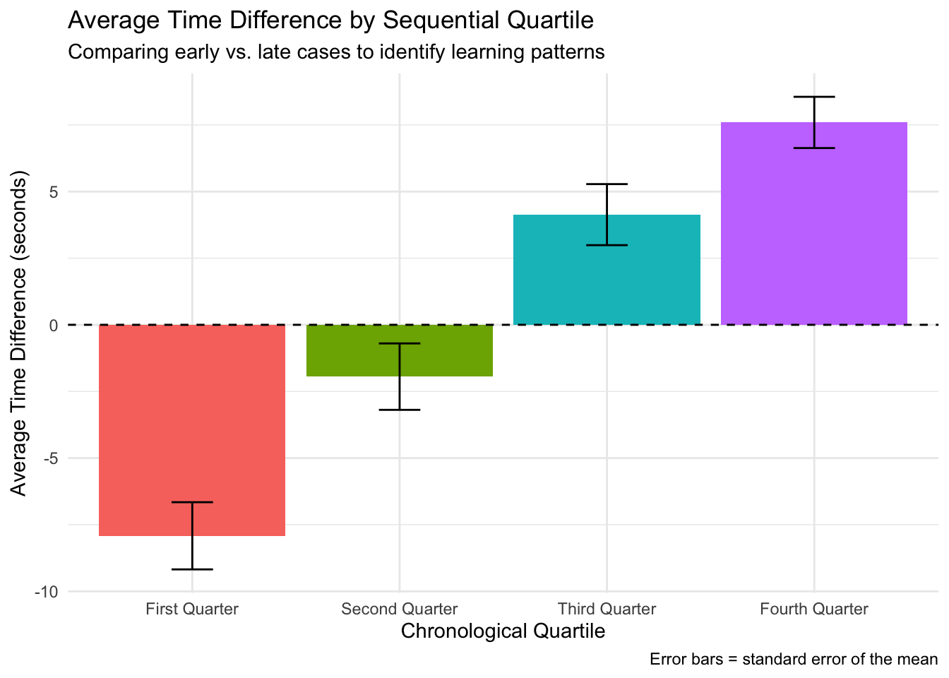
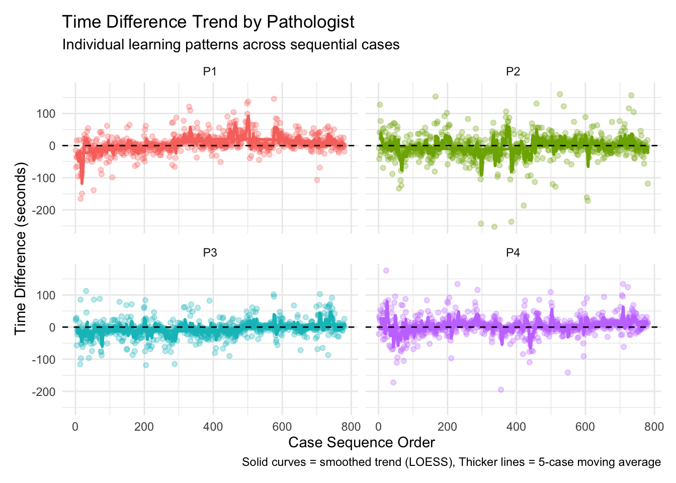
Understanding Learning Effects in Pathologist-AI Interaction The Time Efficiency and Learning Effects analysis helps us understand whether pathologists become more efficient with AI tools over time as they gain experience. This analysis examines several key aspects of the learning process:
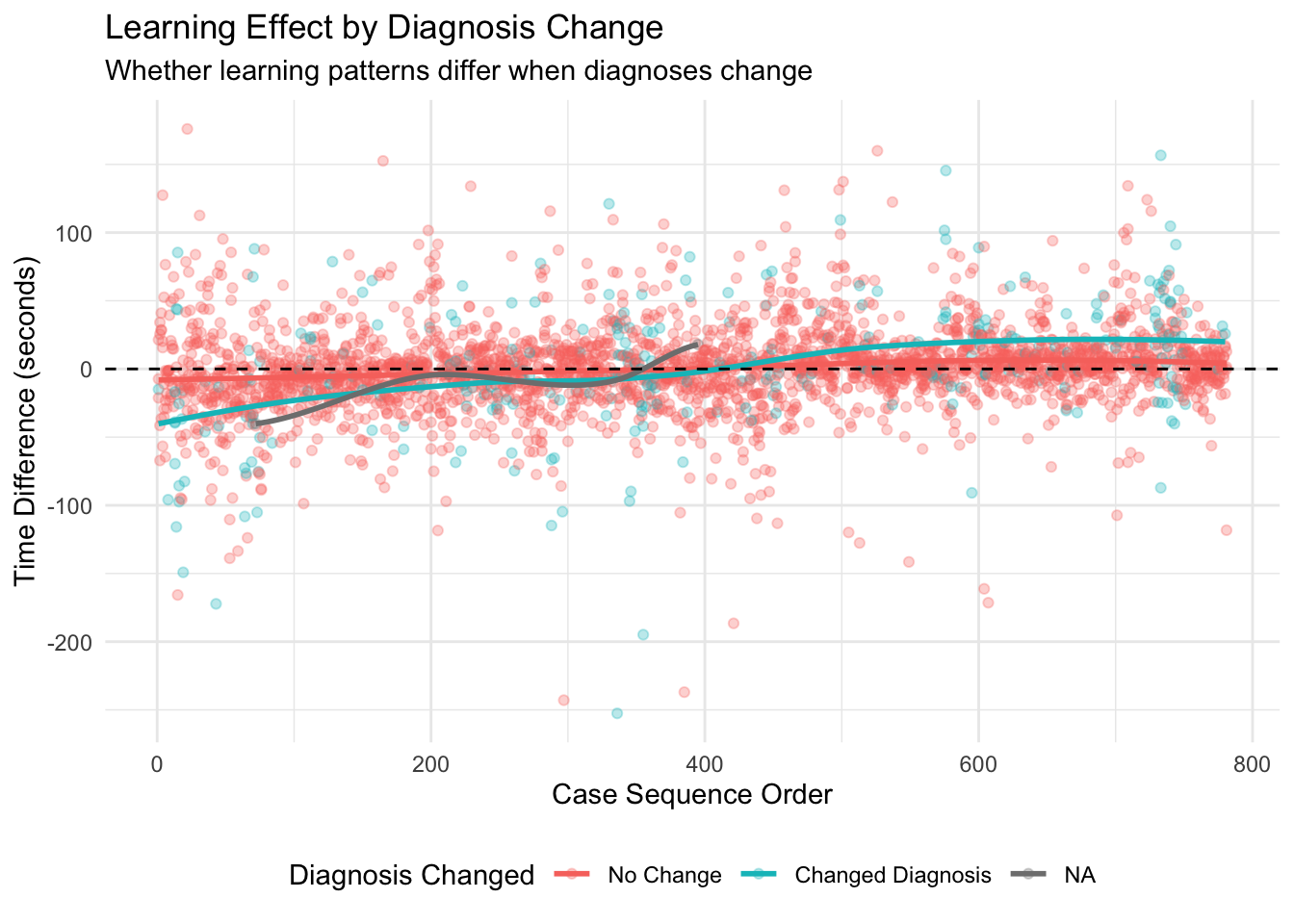
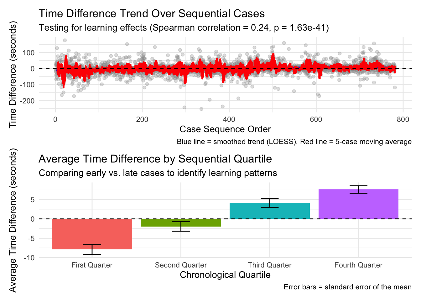
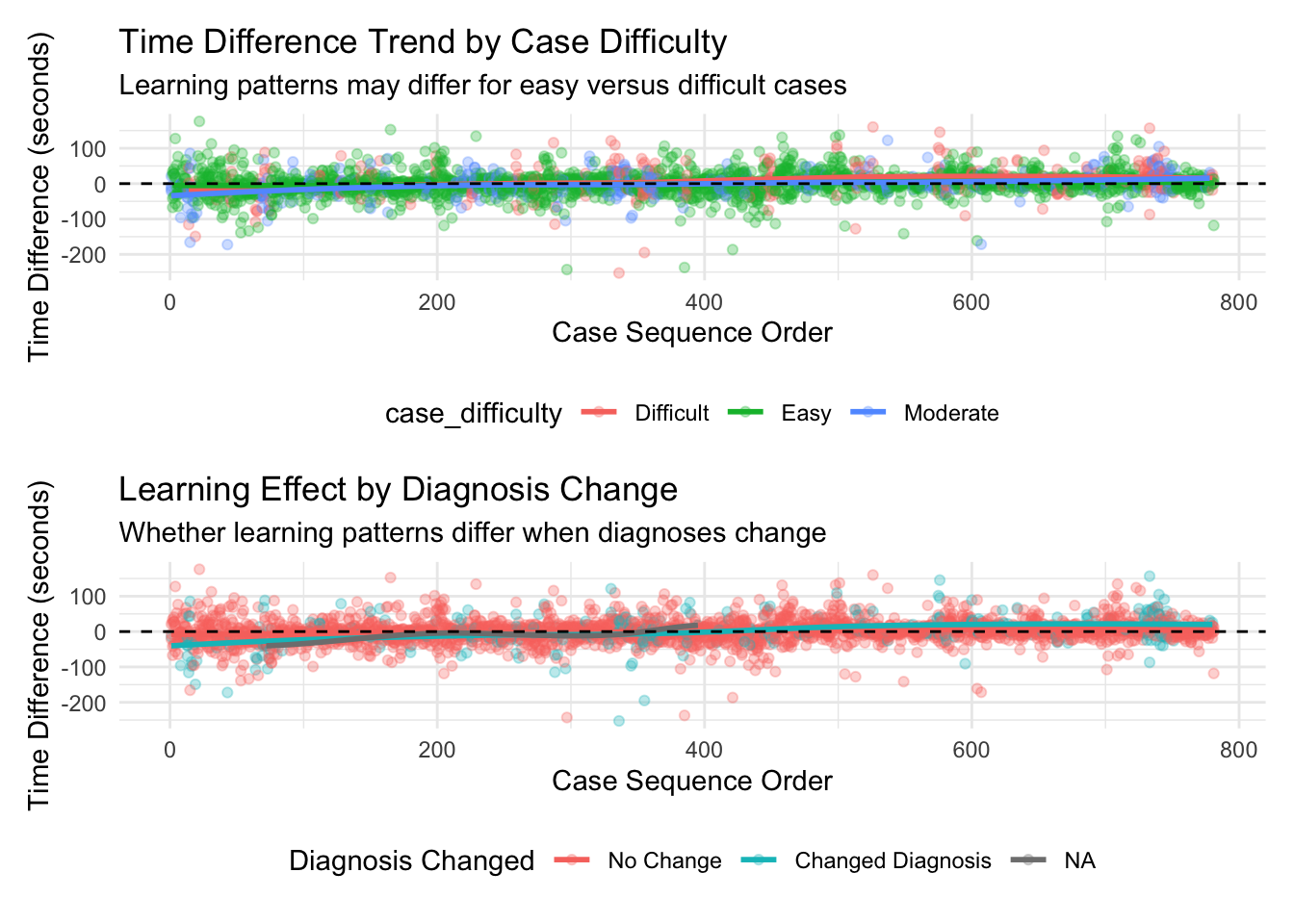
Overall Learning Trend: By ordering cases chronologically and analyzing how time differences change over sequential cases, we can identify whether there’s a general trend toward increased efficiency. The Spearman correlation test provides a statistical measure of this relationship, while the visualized trend line shows the pattern visually. Individual Pathologist Learning: Different pathologists may adapt to AI assistance at different rates. By examining learning effects for each pathologist separately, we can identify which pathologists demonstrate stronger learning patterns and which might benefit from additional training or support. Learning by Case Difficulty: Learning effects may vary depending on case difficulty. Pathologists might show stronger learning patterns for easy cases initially, with improvements on difficult cases coming later as they gain confidence with the AI tool. Alternatively, the greatest time savings might emerge for difficult cases where AI provides the most valuable assistance. Chronological Quartile Analysis: By dividing cases into chronological quartiles (first 25%, second 25%, etc.), we can directly compare early versus late performance to see if efficiency improvements are evident. This approach is less sensitive to outliers or non-linear patterns than correlation analysis. Learning and Diagnosis Changes: The relationship between learning effects and diagnosis changes is particularly important. This analysis shows whether learning curves differ when pathologists change or maintain their diagnoses after seeing AI results. This might reveal whether pathologists become more efficient at incorporating AI input into their decision-making process.
The moving averages (red lines) in the visualizations provide a clearer picture of the trends by smoothing out case-by-case variations, while the LOESS smoothed curves (blue lines) help identify broader non-linear patterns in the learning process. The results from this analysis can help inform:
How much exposure to AI tools pathologists need before reaching optimal efficiency Whether additional training interventions are needed at specific points in the learning curve If certain types of cases benefit more from extended experience with AI How to set realistic expectations for time savings when implementing AI in pathology workflows
By understanding these learning effects, healthcare systems can better plan for the introduction of AI tools, including training requirements, expected productivity changes, and transition periods needed before optimal efficiency is achieved.
Understanding the “Average Time Difference by Sequential Quartile” Plot This plot reveals an important pattern in how pathologists’ efficiency with AI assistance changed over time as they gained more experience using the AI tool. What the plot shows: The plot displays how the time difference between AI-assisted diagnoses and non-AI diagnoses changed across four chronological periods (quartiles) of cases:
X-axis: Shows the sequence of cases divided into four equal time periods (First Quarter through Fourth Quarter) Y-axis: Shows the average time difference in seconds (AI-assisted time minus non-AI time) Bars: Each colored bar represents the average time difference for that quartile Error bars: Indicate the statistical reliability of the averages (standard error of the mean) Dashed line at zero: Reference point where there’s no time difference between AI and non-AI methods
The pattern revealed: The plot shows a striking progression across the four quartiles:
First Quarter: Significant negative time difference (around -8 seconds) - pathologists were notably faster when using AI during their initial cases Second Quarter: Still negative but closer to zero (around -2 seconds) - a smaller time advantage when using AI Third Quarter: Positive time difference (around +4 seconds) - pathologists actually became slower with AI Fourth Quarter: Larger positive time difference (around +7 seconds) - pathologists took even more time with AI in their later cases
What this means: This pattern reveals a reverse learning effect - rather than becoming more efficient with AI over time (as might be expected), pathologists showed a consistent trend toward taking more time with AI assistance as they gained experience. Possible explanations include:
Pathologists may have initially used AI recommendations with minimal review but became more thorough in evaluating AI output as they gained experience They might have developed a more comprehensive approach to incorporating AI input, taking time to compare their own findings with the AI’s suggestions Over time, pathologists might have changed their workflow to leverage AI information more extensively, leading to a more time-consuming but potentially more thorough diagnostic process The error bars not crossing zero suggest these differences are statistically meaningful, not random variation
This finding is particularly important when implementing AI systems in pathology, as it suggests the relationship between experience and efficiency might be more complex than simply “more practice leads to faster performance.”
# A tibble: 4 × 6
  quartile_label mean_without_AI se_without_AI mean_with_AI se_with_AI n_cases
  <fct>                    <dbl>         <dbl>        <dbl>      <dbl>   <int>
1 First Quarter             54.8         1.25          46.9      1.23      784
2 Fourth Quarter            34.7         0.841         42.3      0.971     780
3 Second Quarter            43.7         1.08          41.7      1.09      780
4 Third Quarter             44.3         1.08          48.5      1.20      780
# A tibble: 8 × 5
quartile_label n_cases ai_status time se
<fct> <int> <fct> <dbl> <dbl>
1 First Quarter 784 Without_AI 54.8 1.25
2 First Quarter 784 With_AI 46.9 1.23
3 Second Quarter 780 Without_AI 43.7 1.08
4 Second Quarter 780 With_AI 41.7 1.09
5 Third Quarter 780 Without_AI 44.3 1.08
6 Third Quarter 780 With_AI 48.5 1.20
7 Fourth Quarter 780 Without_AI 34.7 0.841
8 Fourth Quarter 780 With_AI 42.3 0.971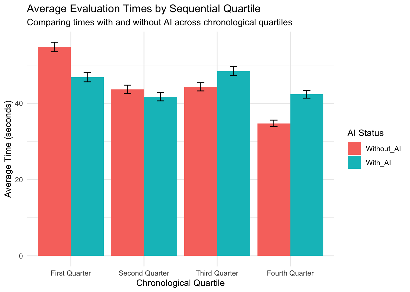
Understanding Pathologist Evaluation Times with AI Assistance: A Chronological Analysis Looking at the image and data table, we can observe a fascinating pattern in how pathologists’ evaluation times changed as they gained experience working with AI assistance. Key Findings Without AI Evaluation Times (Red Bars)
First Quarter: 54.77 seconds Second Quarter: 43.65 seconds Third Quarter: 44.32 seconds Fourth Quarter: 34.73 seconds
Pattern: Pathologists became progressively faster without AI over time, with a substantial 36.6% decrease in evaluation time from first to fourth quarter. This suggests a strong learning effect where pathologists became more efficient with the standard evaluation process as they gained experience. With AI Evaluation Times (Teal Bars)
First Quarter: 46.86 seconds Second Quarter: 41.71 seconds Third Quarter: 48.46 seconds Fourth Quarter: 42.33 seconds
Pattern: AI-assisted evaluations follow a non-linear pattern - initially becoming faster (second quarter), then slowing down significantly (third quarter), before slightly improving again (fourth quarter). Relationship Between AI and Non-AI Evaluations
First Quarter: AI provides a significant time advantage (-7.91 seconds, ~14.4% faster) Second Quarter: AI maintains a small time advantage (-1.94 seconds, ~4.5% faster) Third Quarter: AI becomes slower than non-AI (+4.14 seconds, ~9.3% slower) Fourth Quarter: AI shows the greatest time disadvantage (+7.60 seconds, ~21.9% slower)
Interpretation of These Results
Learning Effects: The consistent improvement in non-AI evaluation times indicates pathologists developed greater expertise and efficiency with the basic task over time. This is a classic learning curve. Changing Relationship with AI: The evolving relationship with AI suggests pathologists’ approach to AI assistance changed dramatically:
Initial AI Benefit: Pathologists likely accepted AI assistance at face value in early cases, using it to expedite their process. Developing Critical Assessment: Over time, pathologists may have developed a more comprehensive and critical approach to AI assistance, spending additional time comparing their own findings with AI suggestions. Methodology Evolution: By the fourth quarter, pathologists were remarkably fast without AI but maintained a more deliberate pace with AI, suggesting they incorporated AI into their workflow in a more thorough but time-consuming manner.
Sample Size Consistency: With approximately 780-784 cases per quartile, these results are based on substantial data, and the small standard errors (0.84-1.25) indicate the trends are statistically meaningful.
Practical Implications These findings challenge the assumption that AI tools automatically lead to time savings. Instead, they suggest that pathologists’ relationship with AI evolves over time from:
Initial “time-saving tool” → More comprehensive “decision support system”
This evolution may result in higher quality assessments that take longer but potentially offer greater accuracy or confidence. The results highlight that implementing AI in clinical workflows requires understanding these temporal dynamics rather than expecting immediate and sustained efficiency gains.